Training extremely large neural networks across thousands of GPUs.

Over the past few years, we've seen an incredible rate of scaling when it comes to training deep neural networks. Today's large language models, for instance, require an immense amount of compute and data to reach state of the art performance.

This scale has been made possible by techniques that allow us to distribute the training of these neural networks across a large cluster of computers, all working in concert to apply gradient descent optimization to a model at massive scale.

In this blog post, we'll discuss techniques such as data and model parallelism which allow us to distribute the model training process across a large cluster of machines.

First, let's revisit the basics

Before we dive into distributed training techniques, let's quickly refresh on the fundamentals of how a neural network is trained. Neural networks are effectively defined by a set of parameterized transformations of our data in order to map the input data to an expected output. We start off with randomly initialized parameters and iteratively refine their values through a gradient descent optimization process.

This gradient descent optimization requires us to define a loss function which describes how close the model's actual output values are to the expected output. We can then compute the partial derivative of our loss function with respect to each parameter in the model (collectively referred to as the gradient) to describe how changes to our model parameters would affect the computed loss. Using this information, we make small updates to each parameter in the model in the direction that would result in a lower value to our computed loss. The magnitude of our update to each parameter is dictated by a learning rate, which effectively controls how "fast" we're able to converge on an optimal set of parameters.

Scaling training to larger batches

In practice, instead of using the entire dataset to compute the gradient during each optimization step, we typically use mini-batches of data, which allows for more frequent updates to our model while still providing a good approximation of the overall gradient.

Smaller batches provide noisier estimates of the gradient; which can be faster to compute but may require more optimization steps to converge on a target loss value. Larger batches, on the other hand, give us a better approximation of the true gradient (leading to smoother optimization dynamics and allowing for us to use a higher learning rate) at the cost of being more expensive to compute per batch.

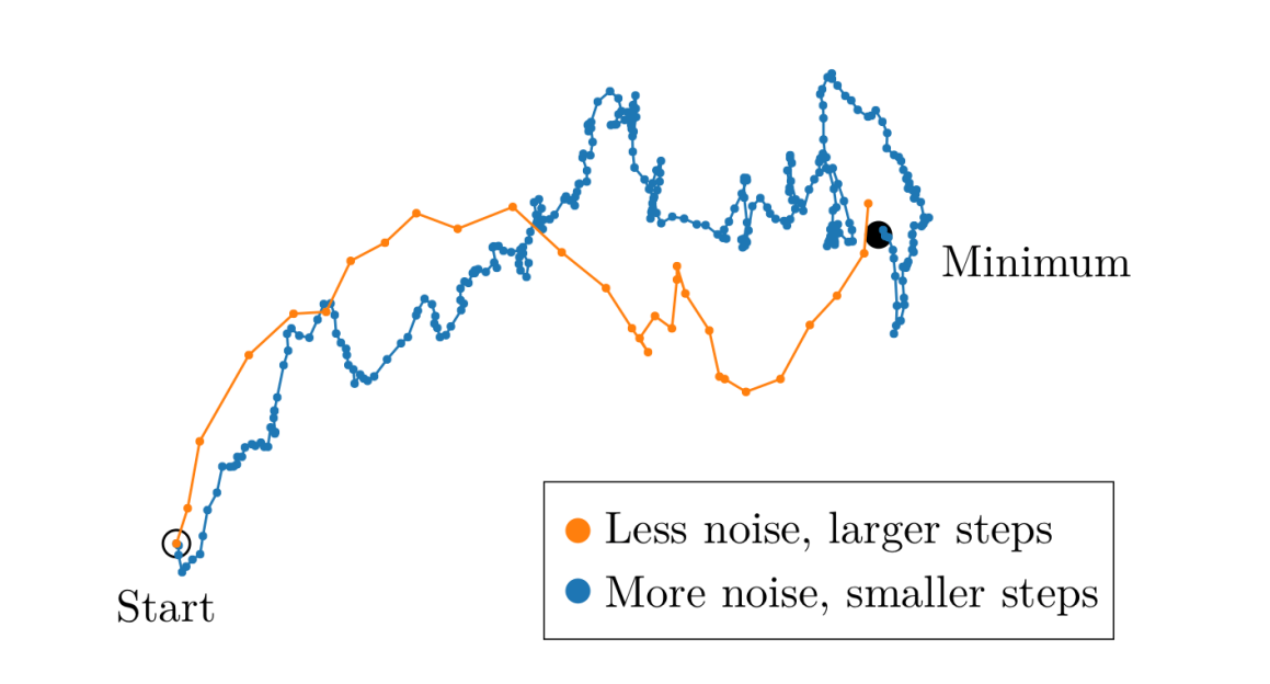
Moreover, as you increase the batch size you'll hit a point where it gives a very close approximation to the true gradient and increasing the batch size further past this point yields minimal benefit (e.g. it's more expensive to compute but doesn't meaningfully improve the estimate of our gradient). As discussed in An Empirical Model of Large-Batch Training, this transition happens at different batch sizes depending on your dataset and the complexity of your modeling task. The paper also provides some guidelines for determining at what batch size this transition will happen based on the per-sample gradients of your input data.

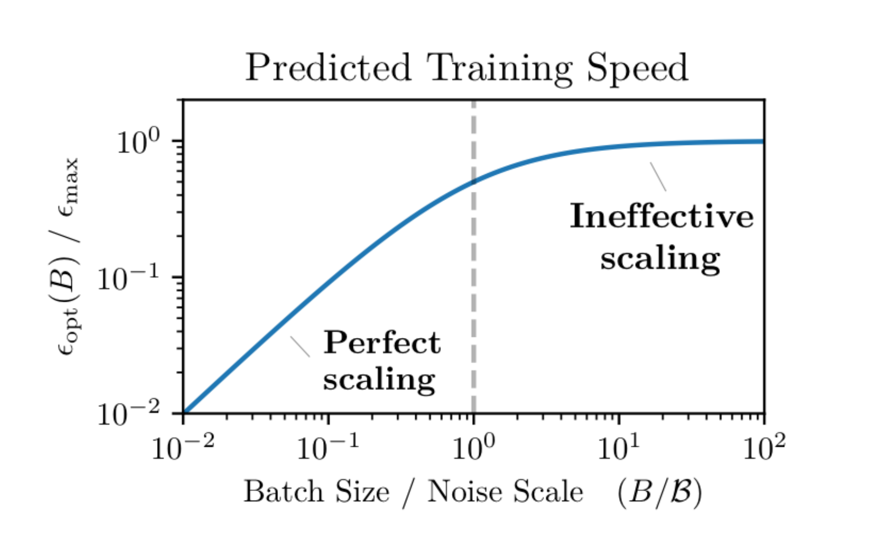
One very impactful result of this paper is that they demonstrate you can often scale to extremely large batches before hitting this transition point for modern day datasets - referencing optimal batch sizes in the tens of thousands of images for ImageNet and up to millions of samples per batch for some reinforcement learning tasks.

It's also important to note that the transition point (referred to as gradient noise scale in the paper) will increase during training as the model's output improves and the gradients become more informative. As a result, you can often increase the batch size as your model trains, such as what was done for Llama 3.1 405B:

...we use an initial batch size of 4M tokens and sequences of length 4,096, and double these values to a batch size of 8M sequences of 8,192 tokens after pre-training 252M tokens. We double the batch size again to 16M after pre-training on 2.87T tokens. We found this training recipe to be very stable: we observed few loss spikes and did not require interventions to correct for model training divergence.

Pushing past the limits of a single machine

If you want to scale your model training to larger batches, however, you're very quickly going to hit the limits of what you can do on a single GPU. Specifically, you'll experience the infamous RuntimeError: CUDA out of memory message that most machine learning engineers know all too well.

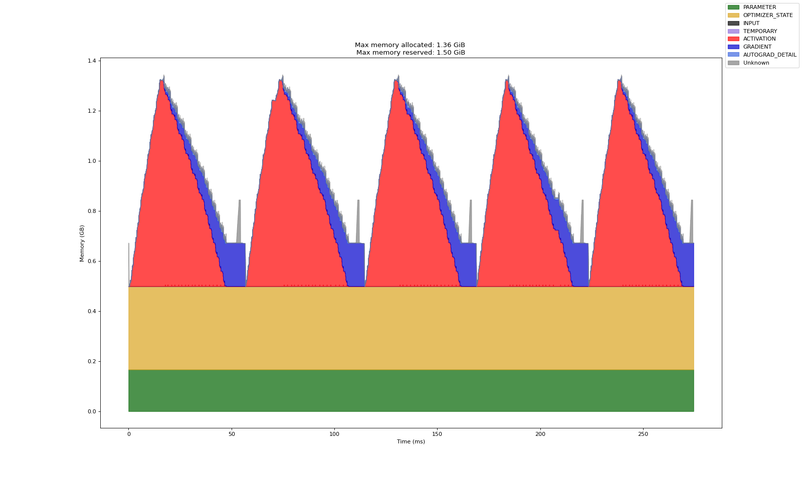
Let's take a second to enumerate the various things that we need to keep in memory while training a model.

• Model parameters: the learnable weights of our model.
• Optimizer states: the exact state that you need to track depends on what optimizer you're using; for example, if you're using AdamW, you'll need to track the first and second momentum estimates in addition to the model parameters.
• Model activations: this will vary based on the architecture of your network and batch size, but can significantly impact memory usage. This information is required for backpropagation to allow us to efficiently compute our gradients.
• Gradients: stored for each parameter of the model, same memory footprint as the model parameters.
• Input data: the batch of input data to be passed to the model, the memory footprint depends on the size and type of data being modeled.

You can look at the overall memory footprint during model training, broken down by category, using PyTorch's memory profiler.

Tricks to reduce memory consumption

There are some tricks that we can employ to squeeze more out of single GPU training or generally reduce the overall memory footprint during training, but these tricks can only take us so far and often trade off reducing memory consumption by requiring more computation.

• Gradient accumulation allows us to scale to larger effective batch sizes by processing smaller batches sequentially. Instead of computing gradients on the full batch at once (which would require storing all activations in memory), we add up the gradients from each small batch before updating the model parameters. This reduces memory usage but requires more forward/backward passes.
• Activation checkpointing allows us to "forget" (i.e. release from memory) some of the activations during the forward pass and recompute the values when needed during the backward pass.
• CPU offloading allows us to transfer some of the state to CPU so we don't have to hold everything in GPU RAM. While CPU operations are slower than GPU operations, moving less frequently accessed data to CPU memory can help us stay within our GPU memory constraints.

All three of these techniques effectively trade extra computation time for reduced memory usage (and there's still a limit to how much they can help in a single GPU setting). In order to efficiently scale up to larger model sizes and ever-growing datasets while still training the model in a reasonable amount of time, we need to distribute our computation over a cluster of machines.

There's two main axes by which we can "split up" the model training process to work across multiple machines:

• Data parallelism: this approach splits the input batch across multiple GPUs, where each GPU has its own copy of the model. Each GPU processes its portion of the data independently, then all GPUs work together to combine their results and update the model. This helps us handle larger batches of data without running into memory limits from input data and activations.
• Model parallelism: when a model is too large to fit on a single GPU (considering parameters, optimizer states, gradients, and activations), we can split it across multiple GPUs in two ways: (1) by dividing the layers across different GPUs, or (2) by splitting individual layers themselves across GPUs.

For the most demanding scenarios, advanced techniques like fully sharded data parallelism combine both approaches to push the limits of what's possible with distributed training.

Data parallelism

Let's dive into how data parallelism works in practice. The core idea is simple: we want to process larger batches of data by spreading the work across multiple GPUs. To make this work in practice, these GPUs need to coordinate during the training process to ensure that each GPU maintains an identical copy of a model while training (resulting in one final trained model at the end of training).

Let's consider an example with 4 GPUs where we want to process a batch of 1024 samples in each step of our training loop:

• Each GPU gets a copy of the model
• The batch is split into 4 chunks of 256 samples each
• Each GPU independently processes its portion of the data
• The GPUs must then coordinate to update the model weights

The first three steps are straightforward - each GPU can compute its predictions and gradients independently. However, if each GPU were to update its model copy using only its local gradients, the models would slowly drift apart as they learn from different portions of data. To keep the models synchronized, we need to communicate the gradient information across all GPUs before updating the model parameters on each device.

To keep our gradients synchronized in data parallel training, we use the all-reduce communication primitive. Here's how it works:

• Each GPU computes gradients on its portion of data
• All GPUs participate in an all-reduce operation to sum the individual local gradients
• Each GPU takes this gradient reduction (sum) and computes the average gradient by dividing by the total number of GPUs
• Each GPU then applies an identical update using this average gradient, keeping the models synchronized

The all-reduce operation has highly-optimized implementations in common distributed communication libraries to minimize communication overhead between GPUs. Instead of every GPU sending its gradients to a central coordinator that averages the gradients and sending the results back to each device (which would create a bottleneck), libraries use clever communication patterns that maximize bandwidth utilization across the available network topology.

Data parallelism allows us to scale up the effective batch size by distributing the input data across multiple GPUs. However, this approach requires storing a complete copy of the model on each GPU. For today's largest models with hundreds of billions of parameters, a single GPU simply doesn't have enough memory to store the model, making it necessary to distribute the model itself across multiple devices.

Model parallelism

For scenarios where the model is too large to fit on a single GPU, we need model parallelism to distribute the parameters across multiple GPU devices. As we discussed previously, there's two main ways we can split up the model: we can either distribute the various layers across different GPUs (pipeline parallelism) or split individual layers themselves across GPUs (tensor parallelism). Let's examine how each approach works and the trade-offs involved.

Pipeline parallelism

In order to explain pipeline parallelism, let's consider a model architecture with 16 layers. In order to distribute these model parameters across 4 GPUs, we'd place layers 1-4 on GPU0, layers 5-8 on GPU1, layers 9-12 on GPU2 and layers 13-16 on GPU3. For a given input batch during training we'd load the input data on GPU0 and pass it through the first four layers, then we'd take the activations of layer 4 and send it as input to layer 5 on the next GPU, then taking the activations of layer 8 and passing it along until we've reached the end of the network and have a final prediction. From here, we can compute our loss and start the backwards pass.

During the backwards pass, we propagate gradients through our pipelined model as follows:

1. On GPU3 (layers 13-16), we start with the gradient of the loss with respect to the model output $\frac{\partial L}{\partial Y}$. We compute the gradients for each layer on GPU3 and end up with $\frac{\partial L}{\partial A_{12}}$ where $A_{12}$ represents the activation matrix output from layer 12 (input to layer 13).
2. This gradient signal $\frac{\partial L}{\partial A_{12}}$ is then sent to GPU2, which is used to compute gradients for layers 9-12 , ultimately producing $\frac{\partial L}{\partial A_{8}}$ to be sent to GPU1
3. The process continues, with GPU1 using $\frac{\partial L}{\partial A_{8}}$ to compute gradients for layers 5-8
4. Finally, GPU0 receives $\frac{\partial L}{\partial A_4}$ and computes gradients for layers 1-4.

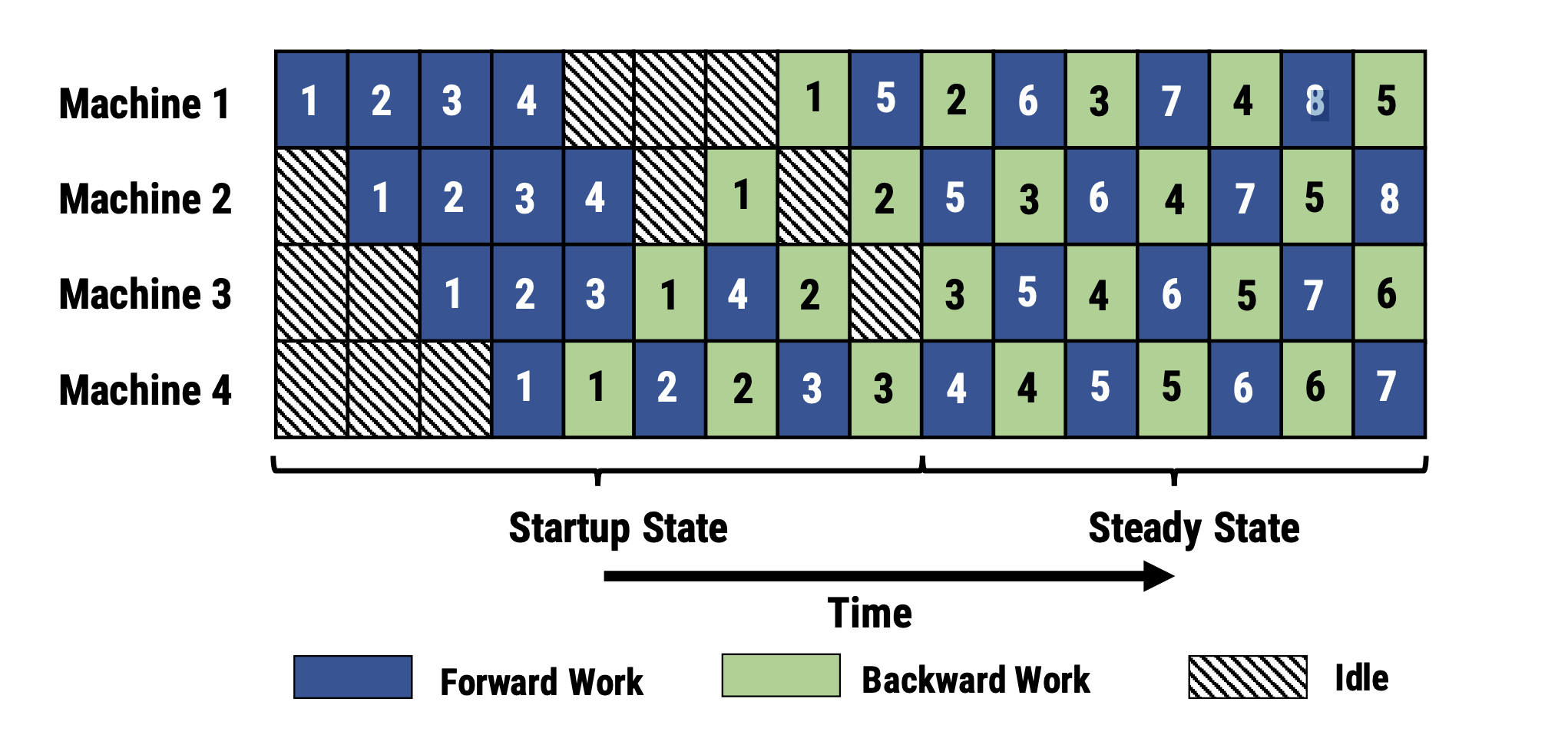
This sequential processing across GPUs creates a challenge in GPU utilization. Consider what happens when processing a batch of data:

1. Initially, only GPU0 is active, processing its layers
2. Then GPU1 starts working, but GPU0 goes back to an idle state
3. Then GPU2 starts, while GPU0 and GPU1 are idle
4. Finally GPU3 processes its layers while the other GPUs wait
5. During the backward pass, the GPUs activate in reverse order, each processing while others remain idle

This leads to significant GPU idle time - a phenomenon known as the "pipeline bubble" because of the gaps in GPU utilization it creates.

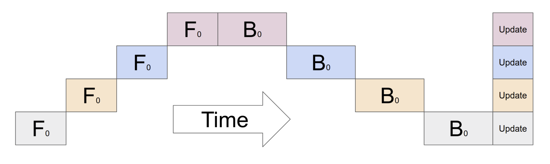
One way to mitigate this issue is to split a batch into multiple micro-batches, allowing different GPUs to work on different micro-batches at the same time. Instead of GPU0 initially processing the entire input batch at once, we'll have it compute a subset (i.e. micro-batch) of the input and pass on those activations to GPU1 to compute the activations of the next layers. This allows GPU0 to compute the next subset of inputs while GPU1 is computing the first subset of inputs. This staggering of computation allows more GPUs to work in parallel, increasing the overall device utilization and reducing the size of the "pipeline bubble". Each device accumulates the computed gradients across all micro-batches before applying an update to the model weights at the end of the pipeline execution.

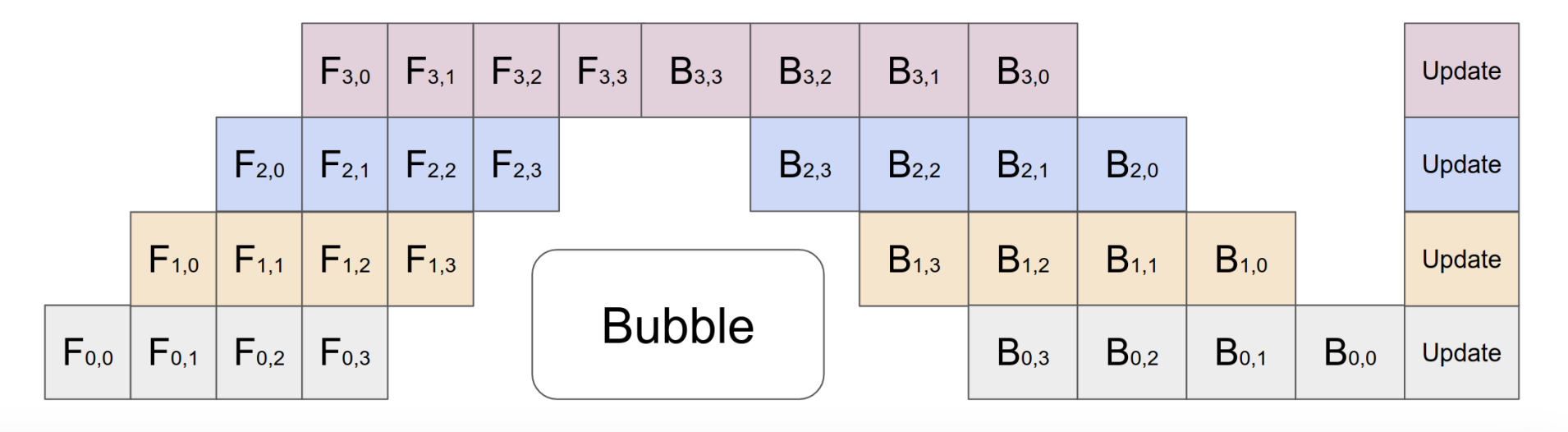
In other variants of pipeline parallelism, model weights can be updated after each micro-batch, resulting in even near-perfect GPU utilization across devices as a result of more dense interleaving of forward and backward passes from the various micro-batches. However, this increased utilization comes at the cost of greater inconsistency as a result of different micro-batches seeing different versions of the model weights.

In summary, pipeline parallelism introduces a simple approach to splitting a large model across GPUs that can be applied to any model architecture without special consideration of layer computations. The main challenge with this approach is ensuring that we can achieve sufficiently high utilization to be able to benefit from the parallel computation.

Tensor parallelism

In order to further increase compute and memory efficiency, tensor parallelism offers an approach which splits the underlying mathematical operations of an individual layer across multiple GPUs. This approach allows easier parallelization of compute (compared to pipeline parallelism) at the cost of increased communication between GPUs.

Let's examine how tensor parallelism works for linear layers, which form the foundation of neural networks and account for the majority of parameters in modern architectures. A linear layer performs the operation $Y = XW$, where:

• $X$ is the input tensor with shape $[\text{batch_size}, \text{input_dim}]$
• $W$ is the weight matrix with shape $[\text{input_dim}, \text{output_dim}]$
• $Y$ is the output tensor with shape $[\text{batch_size}, \text{output_dim}]$

There are two main ways we can partition this matrix multiplication across devices: column and row-wise partitioning.

Column Partitioning

In column partitioning, we split the weight matrix $W$ along its output dimension. This means each GPU stores and computes only a subset of the output features.

Forward Pass:

1. The input $X$ is broadcast to all GPUs
2. Each GPU $i$ computes its portion of the output using its slice of weights: $Y_i = XW_i$
3. The partial outputs are concatenated via an all-gather operation: $Y = [Y_0|Y_1|...|Y_{n-1}]$

Backward Pass:

1. Each GPU receives the slice of output gradients $\frac{\partial L}{\partial Y_i}$ corresponding to its portion of $W$
2. Gradients for the local weights are computed: $\frac{\partial L}{\partial W_i} = X^T \frac{\partial L}{\partial Y_i}$
3. The gradients with respect to $X$ require combining information across GPUs via all-reduce: $\frac{\partial L}{\partial X} = \sum\limits_{i} \frac{\partial L}{\partial W_i}$. These gradients represent how much the activations from the previous layer contributed to the overall loss and are needed to continue the backward pass through earlier layers in the network. 

Row partitioning

In row partitioning, we split the weight matrix $W$ along its input dimension. This means each GPU works with only a subset of the input features.

Forward Pass:

1. Each GPU receives only the portion of $X$ corresponding to its rows of $W$
2. Each GPU computes partial outputs: $Y_i = X_iW_i$
3. The partial outputs are combined via all-reduce: $Y = \sum\limits_{i} Y_i$

Backward Pass:

1. The full gradient $\frac{\partial L}{\partial Y}$ is broadcast to all GPUs
2. Each GPU computes gradients for its local weights: $\frac{\partial L}{\partial W_i} = X_i^T \frac{\partial L}{\partial Y}$
3. Each GPU computes gradients for its portion of $X$: $\frac{\partial L}{\partial X_i} = \frac{\partial L}{\partial Y}W_i^T$. These portions must be combined via all-gather to reconstruct the full $\frac{\partial L}{\partial X}$ tensor needed to continue the backward pass through earlier layers.

Optimizing Communication Through Clever Partitioning

Tensor parallelism requires substantial communication between GPUs, but this overhead can be minimized through careful choices in how we partition consecutive linear layers, as discussed in Megatron-LM: Training Multi-Billion Parameter Language Models Using Model Parallelism where this technique was first introduced.

Consider a sequence of two linear layers with a nonlinear activation function (like GeLU) between them:

1. If we use column partitioning (split weights along the output dimension) for the first layer, each GPU can independently apply the activation function to its portion of the output
2. By then using row partitioning (split weights along the input dimension) for the second layer, each GPU can directly consume its local activations without requiring any communication
3. Finally, we can apply an all-reduce across the devices to combine the final outputs

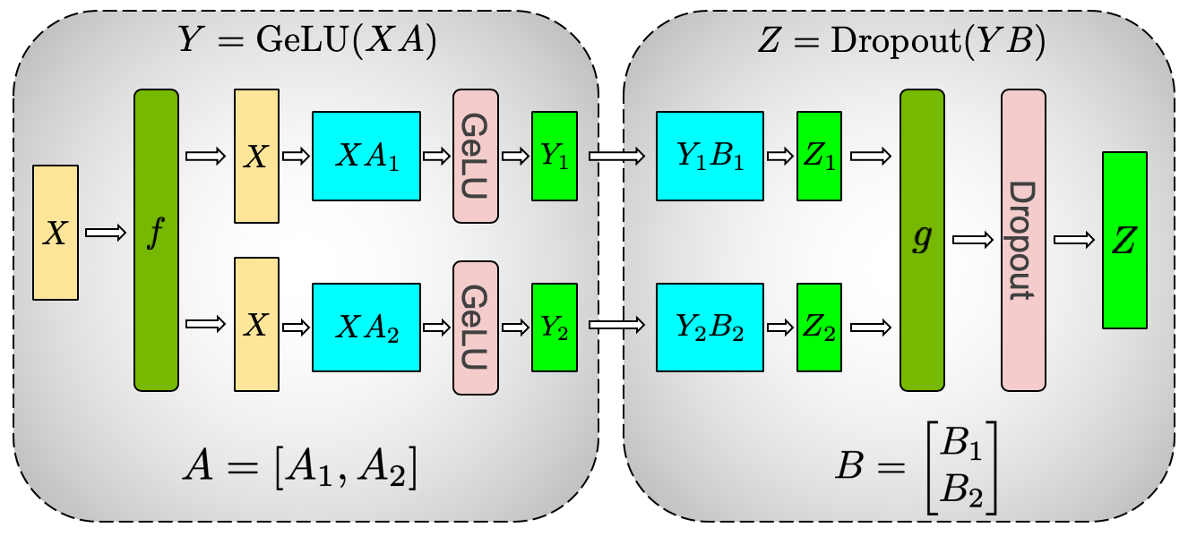
In this scenario, we only need a single all-reduce operation $g$ in the forward pass (to combine the results after the second linear layer) and a single all-reduce operation $f$ in the backward pass (to compute gradients with respect to the first layer's input activations), overall reducing the number of synchronization points by 50% compared to a naive implementation.

Putting it all together

The parallelization strategies we've discussed offer complementary approaches for distributed training that can be combined to maximize training efficiency and scale. However, because these techniques have different communication patterns, the optimal balance and configuration of the different types of parallelism are influenced by your training cluster's network topology.

Modern GPU clusters typically have a hierarchical network structure: GPUs within a node are connected by very high-bandwidth links (like NVLink), while cross-node communication happens over relatively slower network connections (like InfiniBand). For example, Llama 3.1 405B was trained using:

...up to 16K H100 GPUs, each running at 700W TDP with 80GB HBM3, using Meta's Grand Teton AI server platform. Each server is equipped with eight GPUs and two CPUs. Within a server, the eight GPUs are connected via NVLink... each rack hosts 16 GPUs split between two servers and connected by a [network switch] … 192 such racks are [connected] to form a pod of 3,072 GPUs … eight such pods within the same datacenter building are [connected] to form a [total cluster size] of 24K GPUs.

Taking this typical hierarchical network topology into consideration:

• Data parallelism helps us process larger batches by distributing them across many nodes. Since it only requires synchronization during gradient averaging, it remains efficient even with slower cross-node communication.
• Tensor parallelism works best for GPUs with high-speed interconnects, making it ideal for splitting large matrix operations across GPUs within the same node where frequent communication won't become a bottleneck.
• Pipeline parallelism provides an efficient way to split model layers across nodes, minimizing cross-node communication by only needing to pass activations between sequential stages.

Continuing with our example, we can see that Llama 3.1 405B was trained using tensor parallelism of 8, pipeline parallelism of 16, and data parallelism ranging from 8 to 128 as the researchers adjusted the batch size during training. At its peak, the model training was distributed across 16,384 GPUs.

Conclusion

Data, pipeline, and tensor parallelism have enabled researchers and engineers to push the limits of model training to an incredible scale resulting in some seriously impressive capabilities. In addition to these foundational techniques, we've also seen techniques introduced such as context parallelism (for training on long sequence lengths) and expert parallelism (for training sparse models) in order to further improve the scale and efficiency of training state of the art models.

Moreover, these innovations aren't slowing down – the GPU hardware for training gets better every year and new algorithmic improvements (such as DualPipe introduced in DeepSeek-V3 Technical Report) continue to improve the efficiency of large training runs.

References

Papers

• PyTorch Distributed: Experiences on Accelerating Data Parallel Training
• GPipe: Easy Scaling with Micro-Batch Pipeline Parallelism
• PipeDream: Fast and Efficient Pipeline Parallel DNN Training
• Megatron-LM: Training Multi-Billion Parameter Language Models Using Model Parallelism
• Efficient Large-Scale Language Model Training on GPU Clusters Using Megatron-LM
• The Ultra-Scale Playbook: Training LLMs on GPU Clusters
• The Llama 3 Herd of Models

Talks

• Model vs Data Parallelism in Machine Learning | Mark Saroufim
• Distributed Data Parallel in PyTorch Tutorial Series
• Efficient Large-Scale Language Model Training on GPU Clusters Using Megatron-LM | Jared Casper
• Fully Sharded Data Parallel (FSDP) and Pipeline Parallelism in 3D with Vision Pro | Will Falcon